Starting Multiple eCognition Clients
You can start and work on multiple eCognition Developer clients simultaneously; this is helpful if you want to open more than one project at the same time. However, you cannot interact directly between two active applications, as they are running independently – for example, dragging and dropping between windows is not possible.
Default View
eCognition Developer offers two different layouts with predefined user interfaces. A layout provides a selection of tools and user interface elements typically used for image analysis within a commercial and scientific domain: Switch between the data management layout and the ruleset development layout.
However, most tools and user interface elements that are hidden by default are still available via View > Toolbars or View > Customize.
- The Main View displays the image file. Up to four windows can be displayed by selecting Window > Split from the main menu or two windows for Split Vertically or Split Horizontally. You can assign different view settings for an image to each window. The image can be enlarged or reduced using the Zoom functions on the main toolbar (or from the View menu > Display mode).
- View Settings
 : In this dialog you can add image, vector and point cloud layers via drag and drop and edit the according view settings. Toggle between detailed layer properties, switch between grayscale and RGB mixing or - open the 3D toolbar for point cloud data. The upper pane allows individual layer settings, while the lower pane shows global view settings for the respective data type.
 - Process Tree
 : eCognition Developer uses a cognition language to create ruleware. These functions are created by writing rule sets in the Process Tree window
 - Class Hierarchy tab
 : Image objects can be assigned to classes by the user, which are displayed in the Class Hierarchy window. The classes can be grouped in a hierarchical structure, allowing child classes to inherit attributes from parent classes (see Class Hierarchy Concepts)
 - Object Information tab
 : This window provides information about the characteristics of image objects (see Object Information)
 - Feature View tab
 : In eCognition software, a feature represents information such as measurements, attached data or values. Features may relate to specific objects or apply globally and available features are listed in the Feature View window
Default Toolbars and Dialogs
Default Toolbar Buttons
File Toolbar
![]()
The first two buttons allow you to create and save a project, respectively.
![]()
These buttons allow you to create a new workspace, import a project into a workspace, or open an existing workspace.
![]()
This button allows you to open the Import Scenes Dialog and select a predefined import template to fill you workspace with several projects in one go.
Layouts Toolbar
![]()
These buttons allow you to switch between data management layout and ruleset development layout.
Navigate Toolbar
![]()
These toolbar buttons offer direct selection, image panning and a number of zoom options. The zoom level can be entered manually to any user-defined value.
![]()
This drop-down allows for the selection of the map to be displayed in the viewer.
Tools Toolbar
![]()
These buttons allow you to toggle windows on/off:
- workspace
- object information
- object table
- thematic attribute table
- view settings
![]()
This set of buttons allows you to tile and stitch scenes, and create rectangular and polygonal subsets (available in data management layout).
![]()
These buttons allow you start or cancel an analysis of projects on the server.
![]()
This button allows you to toggle the manual editing toolbar on/off.
View Settings dialog
Overview
This dialog controls how image objects, image layers, point clouds, vector layers and regions are displayed in the view.
The upper pane controls the display of individual levels, layers, or clouds, while the lower pane controls global display settings for each available data type.
You can also use the view settings dialog to add data via drag and drop; namely image layers, vector layers, and point clouds.
![]() This button toggles between an expanded or collapsed view of layers, visualizing or leaving out details of loaded layers.
This button toggles between an expanded or collapsed view of layers, visualizing or leaving out details of loaded layers.
![]() These buttons visualize different image layers in grayscale or in RGB. If more than one image layer is loaded, they also allow to shift between layers and their layer mixing.
These buttons visualize different image layers in grayscale or in RGB. If more than one image layer is loaded, they also allow to shift between layers and their layer mixing.
![]() Opens the 3D toolbar (relevant only for point cloud display).
Opens the 3D toolbar (relevant only for point cloud display).
Object level display
Starting eCognition 10, you can display several image object levels at once in the viewer. If this is not suitable change the option either by right-click in the Object Levels section and deactivate Multi-level selection or in Tools > Options > General set Multi-level selection in view settings to 'No' (default setting is 'Yes').
![]()
Upper pane
The Object Levels checkbox in the first line defines for all image object levels:
- the image object level display in general (enable/disable)
- if outlines of objects are displayed
- to draw filled image objects
For the display of individual levels choose between the following options:
- The checkbox allows you to toggle the display of one level on/off completely.
- The outline color selector gives you the option of displaying:
- Class Color - image object outline color is the same as the class color
- No Color - sets the outline color to transparent. This helps for example to visualize more than one image object level: display the outlines of the super-level only and the classification of a sub-level.
- any other color
- The fill selector allows you to choose between class color or feature value (formerly feature view).
- The opacity slider lets you control the opacity/transparency of the filling.
- The context menu enables you to rename or delete an individual level. You can also opt to show or hide all available image object levels (with one click).
Lower pane - Global object level settings
![]()
- The object outline selector lets you choose between display of standard object outlines, polygon (raster) and polygon (smooth). For polygon display you can further opt to display skeletons. Note that skeletons are only displayed in the selected object for performance reasons.
- The class checkboxes allow you to filter the object display by class.
- Finally, you can customize the highlight colors used for selected objects and skeleton display
Image layer buttons
 Single Layer Grayscale
Scenes are automatically assigned RGB (red, green and blue) colors by default when image data with three or more image layers is loaded. Use the Single Layer Grayscale button in the View Settings dialog to display image layers separately in grayscale. To change from RGB to grayscale mode, press the button and the first image layer is shown in grayscale mode. Step through all loaded image layers by using the Show Next/Previous Image Layer button or open multiple views for comparison.
 Three Layers RGB
This button displays the first three layers of your scene in RGB. By default, layer one is assigned to the red channel, layer two to green, and layer three to blue indicated by a small circle in the respective field. View settings can be changed by single click on a circle (removes circle) or an empty field (adds circle).
 Show Previous Image Layer
In Grayscale mode, this button displays the previous image layer. The number or name of the displayed image layer is indicated in the middle of the status bar at the bottom of the main window.
In Three Layer Mix, the color composition for the image layers changes one image layer up for each image layer. For example, if layers two, three and four are displayed, the Show Previous Image Layer Button changes the display to layers one, two and three. If the first image layer is reached, the previous image layer starts again with the last image layer.
 Show Next Image Layer
In Grayscale mode, this button displays the next image layer down. In Three Layer Mix, the color composition for the image layers changes one image layer down for each layer. For example, if layers two, three and four are displayed, the Show Next Image Layer Button changes the display to layers three, four and five. If the last image layer is reached, the next image layer begins again with image layer one.
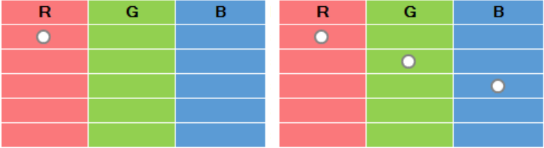
Image Layers - Properties and Settings
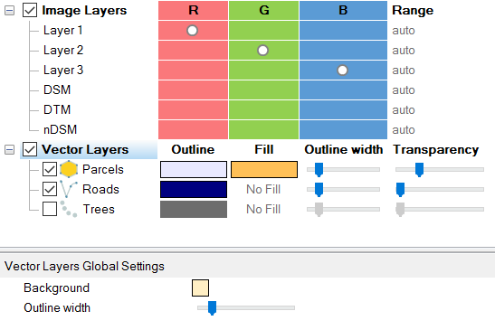
Upper pane - Individual Image Layer Properties
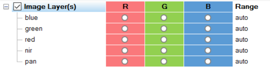
R-G-B: To define the display color of each image layer, you can add a circle for the red, green and blue channels by single click for each layer separately. They are then displayed as additive colors in the view. Any layer without a circle in at least one column is not shown. When creating a new project, the first three image layers are displayed in red, green and blue.
You can change the order of image layers by drag and drop within the Image Layer(s) section.
A right-click on the image layers section opens the context menu where you can select to:
-
Show All or Hide All image layers at once
-
Zoom To Layer (2D) to zoom to the extent of image layers
-
Delete and Rename single image layers
You can also rename an image layer by double click in the view settings dialog and select multiple files for deletion using Ctrl+click.
One layer can be displayed in more than one color, and more than one layer can be displayed in the same color. Change these settings to your preferred by clicking in the respective R, G or B cell.
Range: For the equalization settings (lower pane of dialog) manual, false color (hot metal) and false color (rainbow), you can define the displayed range individually based on the Image Layer Equalization dialog for each image layer. To open the dialog click on the small dots at the end of the line of the image layer you want to adjust (details see Equalization and Image Layer Equalization dialog.)
Changing the view settings only changes the visual display of the image but not the underlying image data – it has no impact on the process of image analysis. You can define the color composition for the visualization of image layers in the view. Additionally, you can choose from different equalizing options. This enables you to better visualize the image and to recognize the visual structures without actually changing them. You can also choose to hide layers, which can be very helpful when investigating image data and results.
Lower pane - global settings for display of image object levels
By changing the Global Settings in the lower pane - all settings in the upper pane are overwritten.
Background: Click on the square to change the background color of the image view.
Raster mode: Select between Image Data and rasterized vectors (used for segmentation). If vector layers are loaded the view visualizes a rasterized version of these layers also used in segmentation algorithms.
Equalization: There are several modes for image equalization stretches. Compare the available methods and choose one that gives you the best visualization of the objects of interest. Equalization settings are stored in the workspace and applied to all projects within the workspace, or are stored within a separate project. In the Options dialog box you can define a default equalization setting. Select on of the following modes:
- none: No equalization allows you to see the scene as it is, which can be helpful at the beginning of rule set development when looking for an approach. The image layer is displayed without further modification.
- linear: Linear equalization with selectable saturation factor [Range 0-50]. Default value 1.00%. Displays images with a higher contrast than without image equalization.
- standard deviation: This equalization has a default factor of 3.0 and renders a display similar to the linear equalization. Use a parameter around 1.0 for an exclusion of dark and bright outliers [Range 0-10].
- gamma correction: Equalization used to improve the contrast of dark or bright areas by spreading the corresponding gray values [Range 0-5]. Default factor 0.5.
- histogram: The histogram equalization increases the contrast of image layers but can lead to over-stretching. Because intensity values are better distributed on the histogram, it can be helpful in cases where you want to display areas with more contrast. The histogram equalization stretches out the most frequent intensity values, not including all intensities.
- manual: Image Layer Equalization enables you to control equalization in detail for each layer individually.
Select either the Range field in the upper pane of the dialog and insert border values to be displayed. Alternatively you can open the Image Layer Equalization dialog by single click on the small dots at the end of the column. For details see also Image Layer Equalization dialog. - false color (hot metal): is recommended for single image layers with large intensity ranges to display in a color range from black over red to white.
Select either the Range field in the upper pane of the dialog and insert border values to be displayed. Alternatively you can open the Image Layer Equalization dialog by single click on the small dots at the end of the column. For details see also Image Layer Equalization dialog. - false color (rainbow): is recommended for single image layers to display a visualization in rainbow colors. Here, the regular color range is converted to a color range between blue for darker pixel intensity values and red for brighter pixel intensity values.
Select either the Range field in the upper pane of the dialog and insert border values to be displayed. Alternatively you can open the Image Layer Equalization dialog by single click on the small dots at the end of the column. For details see also Image Layer Equalization dialog.
Ignore Range: Activating the Ignore range check-box you can enter a range of values that will be ignored when computing the image statistics for the image equalization. (Only active for Equalizing modes linear, standard deviation, gamma correction and histogram)
This option is useful when displaying e.g. elevation data excluding values and background areas in visualization.
This option is only for image visualization. No data values can also be assigned when creating a project see chapter Assigning No-Data Values in Projects and Workspaces.
Elevation (3D view): With point cloud data loaded and the 3D viewer active, image layers can be activated in the View Settings dialog (upper pane) and are then visualized as a 2D image in the 3D viewer. The default elevation for the image layer is the minimum elevation of all currently displayed point cloud points in the 3D viewer, this corresponds to the lower pane parameter value: -auto-. To change the elevation enter a new height value (in project unit) in this field.
Auto update: This checkbox updates the view with each change of the view settings on the fly. Clear this check box to show the new settings after clicking Apply only. With the Auto update check box cleared, the Discard and Apply buttons become active.
Apply to all views: With this checkbox activated you can apply selected settings to all views at once.
The order of image layers and their aliases can be changed easily in the Source View dialog (View > Source View). To rename a layer alias, you can right-click and select rename or press F2 to enter renaming mode or double-click on a layer alias. Alternatively, go to Process > Edit Aliases > Manage Layer Aliases to change image layer, point cloud, and thematic layer aliases in the Image / Point cloud Layer Alias or Thematic Layer Alias tab.
When loading a rule set into a project, it could happen that multiple layer aliases refer to the same physical image channel. In this case, View Settings will display only one layer alias (the one loaded from the rule set).
Image Layer Equalization dialog
To open the Image Layer Equalization window, select in the lower part of the view settings dialog > tab Image Layers > Image Layer Settings > Equalization > manual. Now in the upper part of the dialog single click on the small dots at the end of the line of the image layer you want to adjust. In this dialog you can define the input range by either setting minimum and maximum values, or dragging the borders with the mouse (yellow lines). The equalization range can be set for each layer individually.
It is also possible to adjust these parameters for all image layers using the mouse with the right-hand mouse button held down in the image view: moving the mouse horizontally adjusts the center value; moving it vertically adjusts the width of the interval. (This function must be enabled in: Tools > Options > Display > Use right-mouse button for adjusting window leveling > Yes).
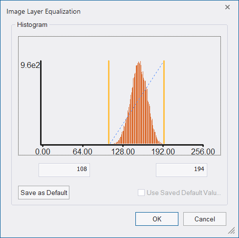
Image equalization is performed after all image layers are mixed into a raw RGB (red, green, blue) image. If, as is usual, one image layer is assigned to each color, the effect is the same as applying equalization to the individual raw layer gray value images. On the other hand, if more than one image layer is assigned to one screen color (red, green or blue), image equalization leads to higher quality results if it is performed after all image layers are mixed into a raw RGB image.
Point cloud properties
The point cloud settings can be changed in the upper and lower pane of the View Settings dialog. Point cloud layers can be shown individually using the respective checkbox of a single point cloud layer. Deactivate the Point Clouds checkbox to hide all point cloud layers in the view or select specific point clouds to hide. You can change the order of point cloud layers by drag and drop within the Point Clouds section.
A right-click on the point cloud layers section opens the context menu where you can select to:
-
Show All or Hide All layers at once
-
Zoom To Layer (2D) to zoom to the extent of point cloud layers in the 2D view
-
Delete and Rename single layers
You can also rename a layer by double click in the view settings dialog and select multiple files for deletion using Ctrl+click.
For details see also User Guide > Projects and Workspaces > Working with Point Clouds.
3D toolbar button ![]() : This button is active on availability once a point cloud layer is loaded to the project. Open this toolbar to select a subset using one of the 3D subset selection buttons and for more visualization options. Subsequently, an additional window is opened where the subset is visualized in 3D (for further details see Navigating in 3D). You can shift the subset when the left view is active, using the left, right, up and down arrows of your keyboard.
: This button is active on availability once a point cloud layer is loaded to the project. Open this toolbar to select a subset using one of the 3D subset selection buttons and for more visualization options. Subsequently, an additional window is opened where the subset is visualized in 3D (for further details see Navigating in 3D). You can shift the subset when the left view is active, using the left, right, up and down arrows of your keyboard.
With the 3D viewer active, image layers can be activated in the View Settings dialog (upper pane) and are then visualized as a 2D image in the 3D viewer. The default elevation for the image layer is the minimum elevation of all currently displayed point cloud points in the 3D viewer (-auto-). Change the elevation of the image layer by using the parameter in the lower pane Elevation (3D view) and enter a new height value (in project unit).
3D vector layers can be displayed in the 3D viewer, supporting 2D and 3D points, lines and polygon outlines (without fill).
The Zoom Scene to Window button  helps you to reset the observer position, all zoom and rotation steps to default.
With point cloud data loaded you can open the toolbar also via View > Toolbars > 3D.
Upper pane of View Settings dialog - Point Cloud Properties
Mode: Choose the visualization mode (see lower pane).
Point Size: Choose the point size in a range between 1 (small) to 10 (large).
Fixed Color: View all points in one selectable color. Only active for Render mode Fixed color.
Lower pane - Point Clouds Global Settings
By changing the Global Settings in this lower pane - all settings in the upper pane are overwritten.
Background: Click on the square to change the background color of the image view. E.g. for the intensity render mode you achieve an improved visualization if you select background color white.
Render mode: Choose the visualization mode:
- Fixed color - view all points in one selectable color
- Classification - color scheme that uses a separate set of colors per class (if available) with selectable colors
- Intensity - gray scale visualization of intensity layer from dark (low intensity) to white (high intensity)
- Color-coded intensity - color scheme gradient from red (low intensity) - yellow - green - to blue (high intensity)
- RGB - visualizes each point based on the original scan colors (optional layer)
- Height - predefined color scheme based on the z value - gradient from blue (low) - green - yellow - to red (high)
The same Render Mode is applied to all point cloud layers and cannot be chosen individually for each point cloud file. However, with the check-box Apply to all views inactive - different point cloud view settings can be chosen for the respective active window (e.g. left window height & right window classification).
Point Size: Choose the point size in a range between 1 (small) to 10 (large).
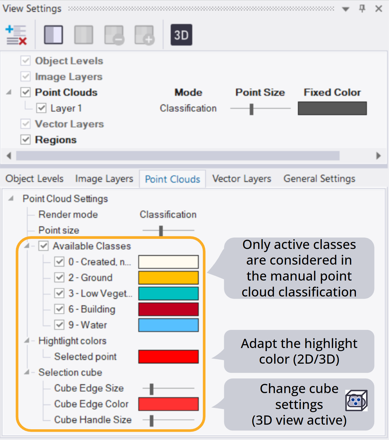
Available Classes: If your point cloud data contains classes you can switch each class on and off individually. In Render mode > Classification you can change the default color for a class by click on the colored rectangle.
Auto update: This checkbox updates the view with each change of the view settings on the fly. Clear this check box to show the new settings after clicking Apply only. With the Auto update check box cleared, the Discard and Apply buttons become active.
Apply to all views: Activate this checkbox to apply the settings to both views.
Vector Layer Display
The vector layer settings can be changed in the upper pane (individual vector layer settings) and lower pane (global settings) of the View Settings dialog. You can change the order of thematic layers by drag and drop.
All thematic layers can be activated and inactivated for display via the Vector Layers checkbox, or individually using the respective checkbox of a single vector layer.
Upper pane - Individual Vector Layer Properties
Outline: Select an outline color.
Outline width: The value for the outline width changes the thickness of the vector outline for all vector layers. (This value is saved in the user settings and therefore applied to different projects.)
Fill: Choose a fill color for polygons.
Opacity: Select the opacity for a vector layer.
Context menu - Vector Layer
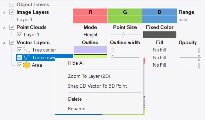
A right-click on the vector layers section opens the context menu where you can select to:
-
Show All or Hide All vector layers at once.
-
Zoom To Layer (2D) to zoom to the extent of a vector layer.
-
Snap 2D Vector To 3D Point to snap a 2D vector layer to a 3D point selected in the view. To snap the vector to another 3D point select a new 3D point and select Snap 2D Vector To 3D Point in the context menu of the vector layer again. Available only for 2D vector layers that do not have elevation information. Snapping a 2D vector to a selected 3D point does not modify vector coordinates and is used only for visualization.
-
Delete and Rename single layers. You can also rename a vector layer by double click in the view settings dialog and select multiple files for deletion using Ctrl+click.
Lower pane - Vector Layers Global Settings
By changing the Global Settings in this lower pane - all settings in the upper pane are overwritten.
Background: Click on the square to change the background color of the image view.
Outline width: The value for the outline width in this lower pane of the dialog changes the thickness of the vector outline for all vector layers. (This value is saved in the user settings and therefore applied to different projects.)
Auto update: This checkbox updates the view with each change of the view settings on the fly. Clear this check box to show the new settings after clicking Apply only. With the Auto update check box cleared, the Discard and Apply buttons become active.
Apply to all views: With this checkbox activated you can apply selected settings to all views at once.
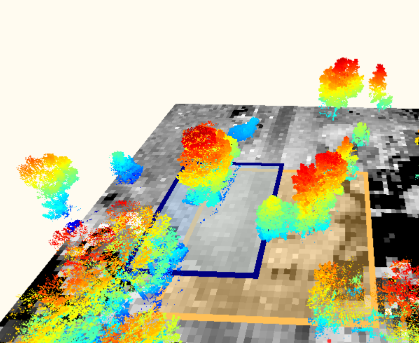
Regions
A region is a defined area that can be used in the domain of algorithms to limit the analysis to a specific area. A region is defined based on a region variable, with values calculated based on different operations, for example using coordinates or the bounding box of an existing image object.
All options are described here
Regions are more flexible than creating a scene subset or working on a map and improve the performance through the limit of the analysis to this defined area.
Since version 10.4 regions are visualized in the main view and 3D view (3D visualization not supported for Mobile Mapping data), and can be handled in the View Settings dialog.
Insert a region using:
-
algorithm - update region (add, edit)
-
View Settings dialog (add, draw, copy, edit, delete, rename)
-
Menu Process > Manage Variables > Regions tab (add, edit, delete, rename)
-
context menu in the main view > right-click > Draw Region
A region can be defined in:
-
2D (X,Y)
-
3D (X,Y,Z)
-
4D (X,Y,Z, T)
-
for time series data (X,Y,T)
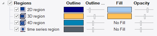
Upper pane - Individual Region Settings
Outline: Select an outline color.
Outline width: Changes the thickness of the outline.
Fill: Choose fill color for a region.
Opacity: Select the opacity for a region.
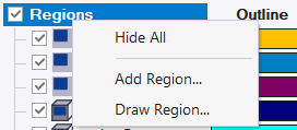
Context menu - Regions
A right-click on Regions opens the context menu:
-
Show All or Hide All regions at once.
-
Add Region... Opens a dialog to insert a new region.
-
Draw Region... Enables the cursor to draw a new region in the main view.
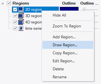
A right-click on one of the inserted regions opens the context menu with the additional options:
-
Zoom To Region zooms to the extent of a region.
-
Copy Region... to duplicate an existing region.
-
Edit Region... to modify an existing region.
-
Delete and Rename single regions. You can also rename a region layer by double click in the view settings dialog and select multiple regions for deletion using Ctrl+click.
Auto update: This checkbox updates the view with each change of the view settings on the fly. Clear this check box to show the new settings after clicking Apply only. With the Auto update check box cleared, the Discard and Apply buttons become active.
Apply to all views: With this checkbox activated you can apply selected settings to all views at once.
More information:
Tutorial - Working with Regions - Update Region algorithm
Algorithm -
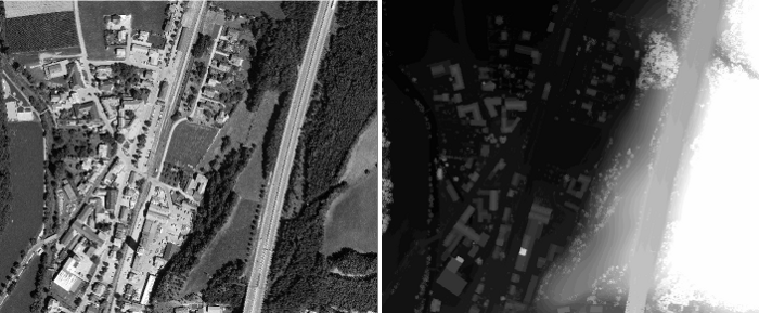
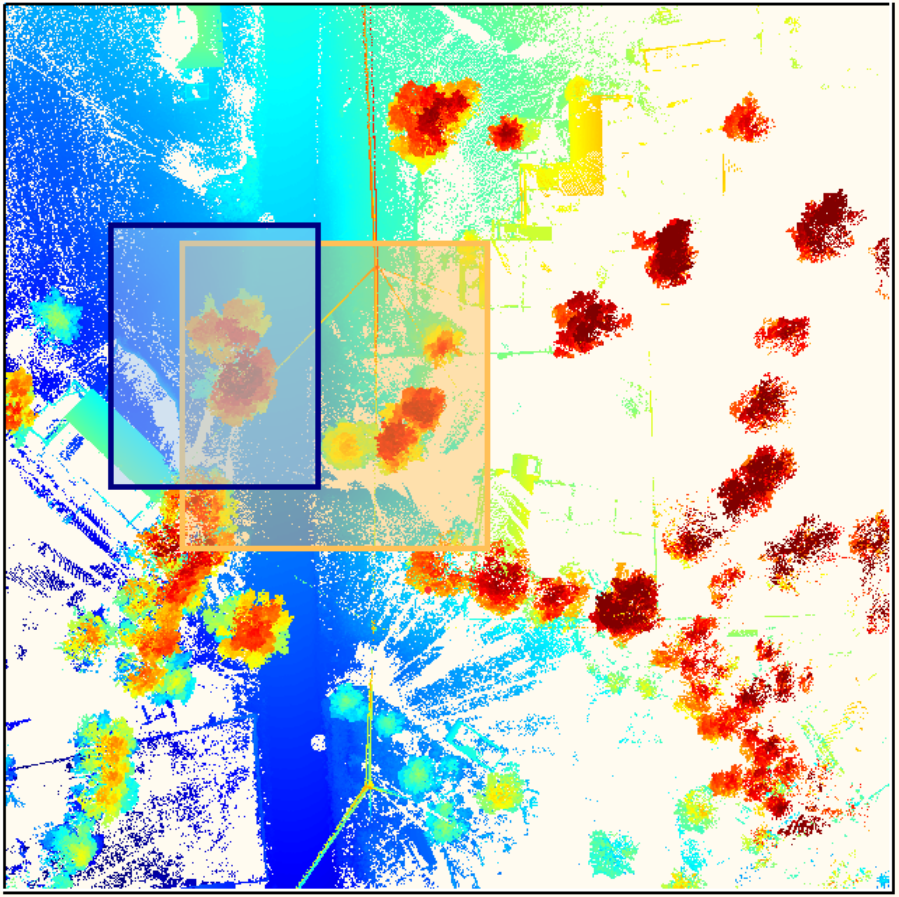
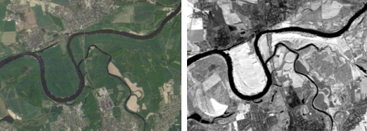
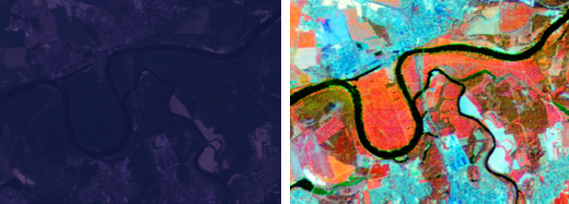
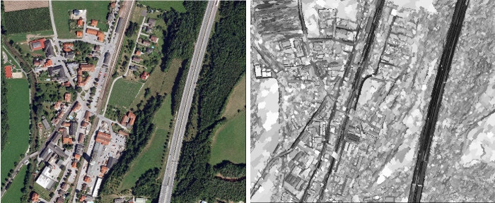
Exemplary View Settings
Compare the following displays of the same scene:
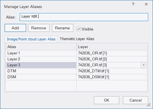
Manage Aliases and Layer Visibility Flag
This dialog allows you to change layer aliases for image layers, point cloud layers, or thematic layers and hide individual layers. Go to Process > Edit Aliases > Manage Layer Aliases > Image / Point cloud Layer Alias (or Thematic Layer Alias) tab to open the dialog.
Select a layer and change its name in the Alias field. Now press the Rename button to apply the new alias. You can also Add new or Remove existing aliases.
In this dialog it is also possible to change the visibility of individual layers and maps: hide a layer by selecting the alias in the left-hand column and unchecking the 'Visible' checkbox.
In addition, you can use the 'assign layer alias' algorithm to rename or assign layer aliases to image, point cloud, or thematic layers.
When loading a rule set into a project, it could happen that multiple layer aliases refer to the same physical image channel. In this case, View Settings will display only one layer alias (the one loaded from the rule set).
Splitting Windows
There are several ways to customize the layout in eCognition Developer, allowing you to display different views of the same image. For example, you may wish to compare the results of a segmentation alongside the original image.
Selecting Window > Split allows you to split the window into four – horizontally and vertically – to a size of your choosing. Alternatively, you can select Window > Split Horizontally or Window > Split Vertically to split the window into two.
There are two more options that give you the choice of synchronizing the displays. Independent View allows you to make changes to the size and position of individual windows – such as zooming or dragging images – without affecting other windows. Alternatively, selecting Side-by-Side View will apply any changes made in one window to any other windows.
A final option, Swipe View, displays the entire image into across multiple sections, while still allowing you to change the view of an individual section.
If you select a different split or turn off the split pane, the view settings of the last active pane are applied.
Docking
By default, the four commonly used windows – Process Tree, Class Hierarchy, Object Information and Feature View – are displayed on the right-hand side of the workspace, in the default Develop Rule Set view. The menu item Window > Enable Docking facilitates this feature.
When you deselect this item, the windows will display independently of each other, allowing you to position and resize them as you wish. This feature may be useful if you are working across multiple monitors. Another option to undock windows is to drag a window while pressing the Ctrl key.
You can restore the window layouts to their default positions by selecting View > Restore Default. Selecting View > Save Current View also allows you to save any changes to the workspace view you make.
eCognition Developer Views
View Layer
To view your original image pixels, you will need to click the View Layer button in the toolbar. Depending on the stage of your analysis, you may also need to select Pixel View (by clicking the Pixel View or Object Mean View button).
In the View Layer mode you can also switch between grayscale and RGB layers using the buttons in the View Settings dialog. To view an image in its original format (if it is RGB), you may need to press the Mix Three Layers RGB button .
![]()
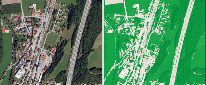
View Classification
Used on its own, View Classification will overlay the colors assigned by the user when classifying image objects (these are the classes visible in the Class Hierarchy window) – the figure below shows the same image when displayed in pixel view with all its RGB layers, against its appearance when View Classification is selected.
Clicking the Pixel View or Object Mean View button toggles between an opaque overlay (in Object Mean View) and a semi-transparent overlay (in Pixel View). When in View Classification and Pixel View, a small button appears bottom left in the image window – clicking on this button will display a transparency slider, which allows you to customize the level of transparency.
Feature View
The Feature View can be used after a first segmentation. You can then select a feature in the Feature tree by double-clicking on it. Image or vector objects are displayed in grayscale according to the feature selected. Low feature values are darker, while high values are brighter. If an object is visualized in red it is not defined for the chosen feature.
For more details see Reference Book > Features - Overview.
Pixel View or Object Mean View
This button switches between Pixel View and Object Mean View.
Object Mean View creates an average color value of the pixels in each object, displaying everything as a solid color. If Classification View is active, the Pixel View is displayed semi-transparently through the classification. Again, you can customize the transparency in the same way as outlined in View Classification.
![]()
Show or Hide Outlines
The Show or Hide Outlines button allows you to display the borders of image objects that you have created by segmentation and classification. The outline colors vary depending on the active display mode:
- In View Layer mode the outline color is blue by default.
- In View Classification mode the outline color of unclassified image objects is black by default.
These two colors can be changed choosing View > Display Mode > Edit Highlight Colors.
- After a classification the outlines take on the colors of the respective classes in View Classification mode.
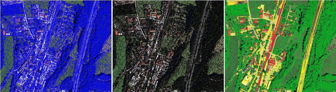
Image View or Project Pixel View
Image View or Project Pixel View is a more advanced feature, which allows the comparison of a downsampled scene (e.g. a scene copy with scale in a workspace or a coarser map within your project) with the original image resolution. Pressing this button toggles between the two views.
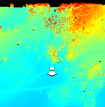
Adding a Color Ramp or a Scale Bar to an Image
The color ramp shows a gradient for single image layers and displays the corresponding layer values. Right-click in the image view, in the context menu select Show Color Ramp Legend to switch the legend on or off. To change the borders of the visualized range please click on the small dots at the end of the line of an image layer you want to adjust (details see Image Layer Equalization dialog).
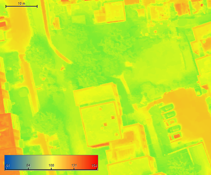
To visualize a scale bar in your image view you can right-click in the image view and choose Show Scale Bar in the context menu or select View > Scale Bar > Visible.
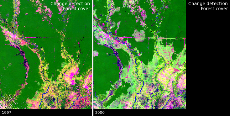
Adding Text to an Image
In some instances, it is desirable to display text over an image – for example, a map title or year and month of a multitemporal image analysis. In addition, text can be incorporated into a digital image if it is exported as part of a rule set.
To add text, double click on the image in the corner of Map View (not the image itself) where you want to add the text, which causes the appropriate Edit Text Settings window to launch. Alternatively, you can also right-click in the image view and choose Edit text (e.g. > Top Left...) in the context menu or select View > Edit text.
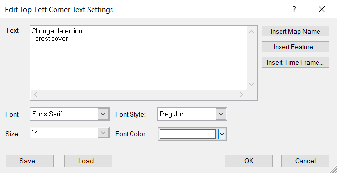
The buttons on the right allow you to insert the fields for map name and any feature values you wish to display. The drop-down boxes at the bottom let you edit the attributes of the text. Note that the two-left hand corners always display left-justified text and the right hand corners show right-justified text.
Text rendering settings can be saved or loaded using the Save and Load buttons; these settings are saved in files with the extension .dtrs. If you wish to export an image as part of a rule set with the text displayed, it is necessary to use the Export Current View algorithm with the Save Current View Settings parameter. Object information is not exported.
Changing the Default Text
It is possible to specify the default text that appears on an image by editing the file default_image_view.xml. It is necessary to put this file in the appropriate folder for the portal you are using; these folders are located in C:\Program Files\Trimble\eCognition Developer \bin\application (assuming you installed the program in the default location). Open the xml file using Notepad (or your preferred editor) and look for the following code:
<TopLeft></TopLeft>
<TopRight></TopRight>
<BottomLeft></BottomLeft>
<BottomRight></BottomRight>
Enter the text you want to appear by placing it between the relevant containers, for example:
<TopLeft>Sample_Text</TopLeft>You will need to restart eCognition Developer to view your changes.
Inserting a Field
In the same way as described in the previous section, you can also insert the feature codes that are used in the Edit Text Settings box into the xml.
For example, changing the xml container to <TopLeft> {#Active pixel x-value Active pixel x,Name}: {#Active pixel x-value Active pixel x, Value} </TopLeft> will display the name and x-value of the selected pixel.
Inserting the code APP_DEFAULT into a container will display the default values (e.g. map number).
Navigating in 2D
The following mouse functions are available when navigating 2D images:
- The left mouse button is used for normal functions such as moving and selecting objects
- Holding down the right mouse button and moving the pointer from left to right adjusts window leveling
- To zoom in and out, either:
- Use the mouse wheel
- Hold down the Ctrl key and the right mouse button, then move the mouse up and down.
Navigating in 3D
If you have loaded point cloud data you can switch to a 3D visualization mode. The according 3D toolbar buttons are only active if point cloud data is loaded to your project.
Point Cloud Navigation and 3D Subset Selection
For adjustment of view settings see Point Cloud View Settings.
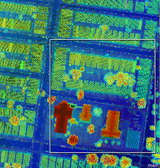
Once you have selected 3D data to be shown in the View Settings dialog you have to choose a 3D subset: Activate the 3D toolbar ![]() and draw a rectangle in the view using the subset button
and draw a rectangle in the view using the subset button  . A new window is opened (right window) where the selected region is visualized in 3D.
Alternatively, you can define a rectangle that lies in the view non-parallel to the window: select the 3 click 3D subset selection button ![]() . This is helpful for the selection of items in the view that are not parallel to the window e.g. for corridor mapping (see 3D Predefined View Toolbar).
. This is helpful for the selection of items in the view that are not parallel to the window e.g. for corridor mapping (see 3D Predefined View Toolbar).
The button Open 3D window with full data extent ![]() opens the full point cloud data extent in the 3D view.
opens the full point cloud data extent in the 3D view.
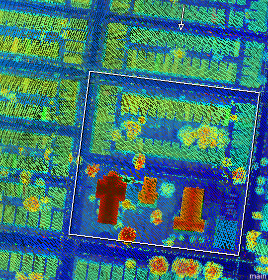
You can shift a selected subset using the left, right, up and down arrows of your keyboard with the left view active.
The 3D subset selection can only be applied if one single window is opened on your screen.
If you are already in 3D mode and split the main window horizontally, the 3D mode is inactivated.
In the main window (left) a small arrow appears that shows the current observer position.
![]()
In the 3D window (right) the following control scheme is applied:
- Left Mouse Button (LMB): While holding down the LMB you can move the mouse up (zoom out) and down (zoom in) to achieve a smooth zooming. This zooming corresponds directly to mouse movement. The cursor turns to a double-pointed arrow.
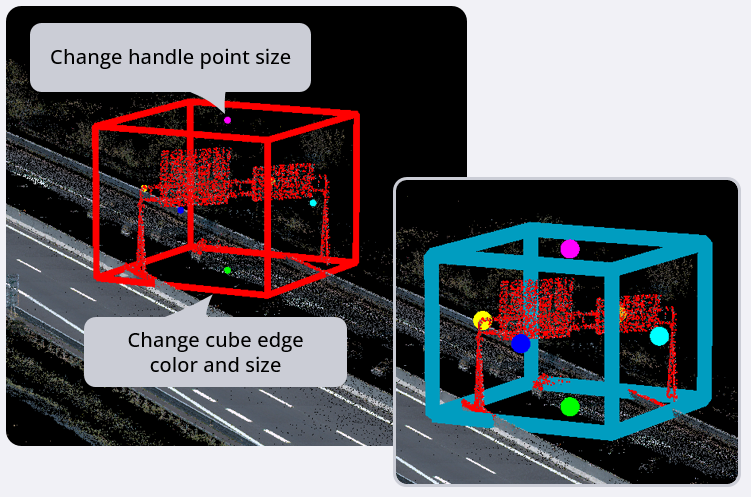
- Left Mouse Button (LMB): With the Object Information window open and point cloud features selected in the Feature view - a single click on a point cloud point shows feature values for the selected point that is visualized as a big red dot. (To change the color go to View > Display mode > Edit highlight colors > Selection color.) When you select a point in the 3D view the same point is highlighted in the main window and vice-versa.
- Right Mouse Button (RMB): While holding down, RMB is used for rotating the point cloud around a center point located in the middle of the selected subset. The cursor turns to a circular arrow and the center point of the subset appears.
Right Mouse Button (RMB) - with activated custom center of rotation : While holding down, RMB is used for rotating the point cloud, now with the center of rotation located at the position where this right mouse button was activated.
 - Mouse Wheel: Rotating the wheel produces a discrete zoom. This zooming is performed in individual steps, corresponding to the rotation of the wheel. The cursor turns to a double-pointed arrow.
- Both LMB and RMB / Press Mouse Wheel: Holding down both the left and right mouse buttons or pressing the mouse wheel enables the user to pan in 3D space. The cursor turns to a hand.
- Alternatively, from the toolbar you can also select the Panning button or the Zoom Out Center and Zoom In Center buttons.
- Zoom Scene to Window button: helps you to reset the observer position, all zoom and rotation steps to default.
![]()
3D Predefined View Toolbar
With 3D data loaded an additional toolbar for predefined settings can be opened via
View > Toolbars > 3D:
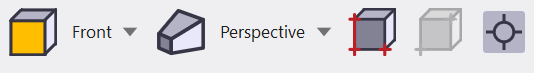
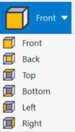
To select a 3D predefined view, choose one of the drop-down commands:
Front, Back, Top, Bottom, Left or Right.
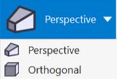
To toggle between different 3D View projections, select either
- Perspective - parallel projected lines appear to converge as they recede in the view or
- Orthogonal - parallel projected lines appear to remain parallel as they recede in the view
 The 3D subset selection button (3-point) lets you define a rectangle by three clicks that can lie in the view non-parallel to the window. This is helpful e.g. for selection of items in the view that are not parallel to the window or for corridor mapping data sets. You can shift the subset using the left, right, up and down arrows of your keyboard with the left view active.
![]() Select a rectangle parallel to the window with the 3D subset selection (2-point) button.
Select a rectangle parallel to the window with the 3D subset selection (2-point) button.
![]() The button Open 3D window with full data extent opens the full point cloud data extent in the 3D view.
The button Open 3D window with full data extent opens the full point cloud data extent in the 3D view.
Activating the Custom center of 3D rotation button while holding down the Right Mouse Button (RMB)rotates the point cloud. The center of rotation is located at the position where this right mouse button was activated.
Point Cloud Editing Toolbar
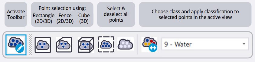
Use this toolbar to assign point cloud points manually to a selected class.
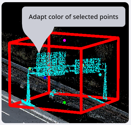
Select the point cloud points in the 2D view based on the rectangle or polygon selection tool or based on a resizable rectangular cuboid or fence selection in the 3D view. Selected points are visualized by default as small red dots.
Choose the appropriate class from the drop-down menu.
Assign the selected points using the classify button. Note that only selected points of the active view are classified. (Change the view settings mode of your point cloud to Classification to see the results.)
 Point cloud editing toolbar - Show or hide the point cloud editing toolbar.
 Rectangle point selection - Select points by drawing a rectangle (2D & 3D view, Shortcut R). All points are selected within the rectangular area that extends into 3D space.
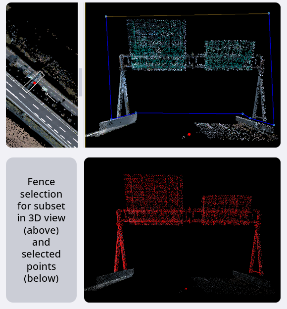
 Fence selection - Select points by drawing a polygon to define the boundaries of an irregular point cloud region . All points are selected within a polygonal area that extends into 3D space. (2D & 3D view, Shortcut P)
 Cuboid point selection - Select points enclosed by a resizable rectangular cuboid (3D view, Shortcut B). Single-click to determine the center point of the cube.
 Select all point cloud points of active classes of the current map (2D & 3D, Shortcut S).
 Clear all selected point cloud points (2D & 3D, Shortcut Ctrl+C).
 Classify selected points of the active view to the class chosen in the drop-down menu (Shortcut C).
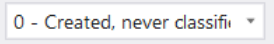 Select point cloud class for classification.
Important:
Press escape (Esc) to exit a selected tool.
You can close a selection polygon (2D and 3D view) by single click on the starting node or by double-click in the view.
Selection in 3D view - Before drawing a rectangle or polygon, position the point cloud in the 3D view so that the points to select are visible.
Additionally, you can select a 3D subset to confine the area of interest and prevent the selection of points beyond this region. Since the selection area may extend beyond your specified boundaries, using the subset selection helps to limit the selection boundary and concentrate your work within a smaller, more focused subset of data.
3D subset selection button (3-point)  3D subset selection (2-point)
If you switch off classes in the lower part of the point cloud view settings dialog - they are not considered in the selection and classification process.
To insert the selection cube, single-click without dragging to determine the center point of the cube. (The cube size is estimated based on the pixel size of your project. The default size is 10 pixels on each axis, but it will always be positioned above or on the lowest point in the point cloud. If the subset is smaller than 10 pixels, the cube will adjust to the size of the subset.)
Time Series - Mobile Mapping - Camera View Data
The map features of eCognition also let you investigate time series or mobile mapping data sets - which corresponds to a continuous film image.
There are several options for viewing and analyzing camera view image data represented by eCognition maps. You can view time series data using special visualization tools.
3D Toolbar - Time Series
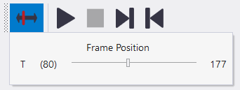
Go to View > Toolbars > Time Series to open the toolbar for the following functionality:
- Frame Navigation - Use this slider to navigate through the frames by selecting a frame position.
- Start/Stop time frame animation - shows the time frames in a loop until you press stop (Ctrl + Space)
- Show next time frame - shows the next time frame starting from this position (Ctrl + Mouse Wheel zoom in or Ctrl + Right)
- Show previous time frame - show the previous time frame (Ctrl + Mouse Wheel zoom out or Ctrl + Left)
The current frame number is displayed in the bottom right corner of the map view - time frame 2 corresponds to T:2.
See also: Working with Mobile Mapping Data
Note that the button Open 3D window with full data extent ![]() is the only option for mobile mapping data, all other subset selection buttons are deactivated.
is the only option for mobile mapping data, all other subset selection buttons are deactivated.
Viewing a Video (Time Series)
Image data that includes a video (time series) can be viewed as an animation. You can also step though frames one at a time.
To view an animation of an open project, click the play button in the Animation toolbar; to stop, click again. You can use the slider in the Time Series toolbar to move back and forth through frames. Either drag the slider or click it and then use the arrow keys on your keyboard to step through the frames.
Shortcuts / Help Keyboard
Following shortcuts are available by default. All shortcut keys can be edited using View > Customize > Keyboard > Press New Shortcut Key.
| Shortcut | Functionality | Related to |
| B | Select points enclosed by a resizable rectangular cuboid in the 3D view. | Point Cloud Editing Toolbar |
| C | Classify selected points to the class chosen in the drop-down menu. | Point Cloud Editing Toolbar |
| Ctrl + A | Add new process in process tree. | Process tree |
| Ctrl + Alt + M | Delete samples of selected classes. | Samples |
| Ctrl + F | Open/Close find & replace window. | Find & Replace |
| Ctrl + H | Shows the histograms of the scene. | Project |
| Ctrl + I | Insert new child process in the process tree. | Process tree |
| Ctrl + M | Open/Close the sample editor. | Samples |
| Ctrl + N | Load an image file and create a new project. | Project |
| Ctrl + P | Activate/Deactivate the panning hand. | Visualization |
| Ctrl + S | Save the currently open project. | Project |
| Ctrl + Shift + P | Open/Close the pan window. | Visualization |
| Ctrl + U | Activate/Deactivate area zoom. | Visualization |
| Ctrl + Enter | Open and edit selected process. | Process tree |
| Ctrl+C | Clear all selected point cloud points (2D & 3D). | Point Cloud Editing Toolbar |
| F1 | Open the html online help. | Help |
| F3 | Open find & replace window/locate next item found in this window. | Find & Replace |
| F5 | Execute selected process in the process tree. | Process tree |
| F6 | Execute selected process on a selected object only. | Process tree |
| F9 | Set a breakpoint on the selected process in the process tree. | Process tree |
| P | Fence selection to select points by drawing a polygon in the 2D or 3D view. | Point Cloud Editing Toolbar |
| R | Select points by drawing a rectangle in the 2D view. | Point Cloud Editing Toolbar |
| S | Select all point cloud points of active classes of the current map (2D & 3D). | Point Cloud Editing Toolbar |
| Shift + F3 | Locate previous item found in find & replace window. | Find & Replace |
Shortcuts grouped by relation:
| Shortcut | Functionality | Related to |
| F1 | Open the html online help. | Help |
| F6 | Execute selected process on a selected object only. | Process tree |
| F5 | Execute selected process in the process tree. | Process tree |
| Ctrl + Enter | Open and edit selected process. | Process tree |
| F9 | Set a breakpoint on the selected process in the process tree. | Process tree |
| Ctrl + A | Add new process in process tree. | Process tree |
| Ctrl + I | Insert new child process in the process tree. | Process tree |
| Ctrl + N | Load an image file and create a new project. | Project |
| Ctrl + H | Shows the histograms of the scene. | Project |
| Ctrl + S | Save the currently open project. | Project |
| Ctrl + M | Open/Close the sample editor. | Samples |
| Ctrl + Alt + M | Delete samples of selected classes. | Samples |
| Ctrl + Shift + P | Open/Close the pan window. | Visualization |
| Ctrl + U | Activate/Deactivate area zoom. | Visualization |
| Ctrl + P | Activate/Deactivate the panning hand. | Visualization |
| Ctrl + F | Open/Close find & replace window. | Find & Replace |
| F3 | Open find & replace window/locate next item found in this window. | Find & Replace |
| Shift + F3 | Locate previous item found in find & replace window. | Find & Replace |
| R | Select points by drawing a rectangle in the 2D view. | Point Cloud Editing Toolbar |
| P | Fence selection to select points by drawing a polygon in the 2D or 3D view. | Point Cloud Editing Toolbar |
| B | Select points enclosed by a resizable rectangular cuboid in the 3D view. | Point Cloud Editing Toolbar |
| S | Select all point cloud points of active classes of the current map (2D & 3D). | Point Cloud Editing Toolbar |
| Ctrl+C | Clear all selected point cloud points (2D & 3D). | Point Cloud Editing Toolbar |
| C | Classify selected points to the class chosen in the drop-down menu. | Point Cloud Editing Toolbar |
